E1 - From Code to Cognition: My AI Exploration Begins

Introduction to AI and LLM - history and basic concepts

1. Introduction

In a world where the term "Artificial Intelligence" (AI) has become ubiquitous, it's crucial to ground my understanding in its foundational aspects. John McCarthy, a luminary in the domain from Stanford University, delved deep into the basic questions surrounding AI in his paper "WHAT IS ARTIFICIAL INTELLIGENCE?". At its core, AI revolves around the science and engineering of creating intelligent machines, especially intelligent computer programs. Human intelligence, on the other hand, is often characterized by our ability to perceive, reason, learn from experience, and adapt to varying situations. People often think AI and human intelligence are the same thing. But even if AI might seem like it's thinking like us, it's actually pretty different in its own ways. That's an important thing to remember!

While AI may often engage in simulations of human intelligence, it's essential to understand that a simulation, by definition, can mimic or act like the real thing but is not the genuine article itself. Thus, AI's reflection of human-like intelligence is a crafted representation, not a genuine replication. Understanding intelligence itself is complex, described by McCarthy as the computational aspect of the ability to achieve goals. The realm of AI research is vast and multifaceted, navigating beyond mere simulations of human intelligence

2. The Evolution of Artificial Intelligence

1950s: The initiation of AI was marked by Alan Turing's Turing Test, a theoretical benchmark for gauging machine intelligence. The core idea was simple: if a machine could converse indistinguishably from a human, it could be termed 'intelligent'. Concurrently, John McCarthy's Lisp emerged as a pioneering language for AI due to its symbolic processing capabilities, representing a shift from mere arithmetic computations to symbolic reasoning.

1960s: The advent of rule-based systems became evident. Joseph Weizenbaum's ELIZA utilized pattern-matching algorithms to replicate human-like interactions, marking an early exploration into Natural Language Processing (NLP). Though rudimentary, it demonstrated that machines could, at a basic level, "understand" and generate human language.

1970s: Expert systems, epitomized by MYCIN, brought forth a new paradigm. MYCIN, using a backward chaining algorithm, diagnosed bacterial infections. It marked an evolutionary step by employing rule-based logic on domain-specific knowledge, showcasing the potential of machines to emulate specialized human decision-making. Concurrently, the Stanford Cart, using basic computer vision algorithms, created the promise of autonomous movement.

1980s: Expert systems further matured. They encapsulated human expertise using a combination of knowledge bases and inference engines. Yet, their rigidity was evident; they were only as good as the rules fed into them. This decade also marked a resurgence of interest in neural networks, especially with the Backpropagation algorithm, which allowed the optimization of weights in multi-layered networks, paving the way for deep learning.

1990s: IBM's Deep Blue, while a hardware marvel, utilized alpha-beta pruning and advanced evaluation heuristics to search through vast chess positions. This marked an evolutionary leap in combinatorial optimization. Simultaneously, Sony's AIBO, a blend of sensors and real-time processing, showcased AI's potential in robotics.

2000s: The DARPA Grand Challenge was emblematic of advancements in sensor fusion and real-time decision-making. Machine learning began to shift from purely supervised paradigms to semi-supervised and unsupervised methods. Techniques like Random Forests, SVMs, and Boosting became predominant, laying the groundwork for more complex architectures.

2010s: The term deep learning became synonymous with AI. DeepMind's AlphaGo combined deep convolutional networks with Monte Carlo Tree Search, marking a significant advancement in reinforcement learning. Architectures evolved from simple feed-forward networks to more complex structures like RNNs, LSTMs, and Transformers. OpenAI's GPT-2's transformer architecture showcased the potential of attention mechanisms, setting new benchmarks in NLP.

2020s: OpenAI's GPT-3 brought zero-shot and few-shot learning into the spotlight, emphasizing the capability of models to generalize from limited data. This evolution underscores a trend: from handcrafted rules to data-driven decision-making, from shallow models to deep, intricate architectures.

3. Basic Terminology and Applications

Artificial Intelligence (AI): AI refers to the capability of a machine to mimic intelligent human behavior. It's a broad field that encompasses everything from robotic process automation to actual robotics.

Machine Learning (ML): ML allows computers to learn from data. Instead of being explicitly programmed to perform a task, the machine uses data and algorithms to learn how to perform the task by itself.

Deep Learning (DL): Deep Learning is a subfield of ML. It's primarily concerned with algorithms inspired by the structure and function of the brain called artificial neural networks. These algorithms are known for processing vast amounts of data, including unstructured data like images and text.

Large Language Models (LLM): LLMs, like GPT-4, are a type of Deep Learning model designed to understand and generate human-like text based on the patterns they've learned from massive datasets. They are particularly known for their ability to generate coherent and contextually relevant sentences over long passages.

Real-world applications: How AI touches our everyday lives:

1. Personal Assistants: Virtual personal assistants, like Siri, Alexa, and Google Assistant, use AI to interpret and respond to user prompts.

2. Recommendation Systems: From Netflix movie suggestions to Amazon product recommendations, these systems use ML algorithms to tailor content to individual user preferences.

3. Autonomous Vehicles: Cars like those from Tesla use a combination of sensors and AI algorithms to drive themselves.

4. Medical Diagnosis: Advanced AI tools can help in diagnosing diseases and conditions from medical imagery with impressive accuracy.

5. Language Translation: Platforms like Google Translate employ Deep Learning models to provide real-time translation across dozens of languages.

6. Financial Trading: AI-powered systems analyze market conditions in real-time to make trading decisions at speeds far surpassing human capabilities.

7. Chatbots and Customer Service: Many websites now have chatbot assistants that can answer user queries in real-time, improving user experience and efficiency.

8. Smart Home Devices: Devices like Nest or Ring use AI to learn user behaviors and preferences, adjusting settings automatically for user convenience.

These applications highlight the extensive reach of AI technologies in various industries and our daily lives.

4. The Backbone of AI: Mathematical Foundations

At the foundation of Artificial Intelligence, there are mathematical principles. These pillars grant AI its strength and capabilities.

4.1. Linear Algebra

Definition:
Linear algebra is a branch of mathematics concerning linear equations, linear functions, and their representations in vector spaces and through matrices. Fundamentally, it deals with vectors, matrices, determinants, and systems of linear equations.

Relevance to AI:
In AI, and particularly in deep learning, linear algebra is crucial. Data, whether they are images, sound, or numerical values, are often represented as vectors or matrices. When processing this data, especially in neural networks, computations are performed using the principles of linear algebra. These computations include operations like matrix multiplication, finding eigenvectors/eigenvalues, and more. The efficiency and scalability of these operations are essential for training large neural networks on vast datasets.

Use case example:
Imagine training a neural network to recognize characters from popular culture.

The image provided, for instance, represents Darth Vader from the Star Wars series. An image can be thought of as a matrix where each entry in the matrix represents the pixel intensity (and possibly color channels). When this image is fed into a neural network, the matrix undergoes various linear algebraic operations, like matrix multiplications, to transform the raw pixel values into a form that the network can use to recognize and classify the character. Through multiple layers and operations, the network might learn to pick up on unique features such as the distinct helmet shape, the pattern of the grille on the mouthpiece, or the silhouette of the cape, which all signal that this could be an image of Darth Vader.

Imagine the image of Darth Vader being represented as a matrix.

# Example Python Code for Matrix-Vector Multiplication related to the Darth Vader image

# Let's assume a simplified 3x3 grayscale image of Darth Vader 
# (in reality, the image would have thousands or millions of pixels, 
# and possibly three channels for RGB)

# Simplified pixel matrix of the image (just an illustrative example)
darth_vader_image = [
    [230, 235, 232],   # top row of the image
    [50, 40, 48],     # middle row representing the darker mask region
    [220, 225, 222]   # bottom row of the image
]

# A sample weight matrix from the first layer of a neural network
weights = [
    [0.1, 0.2, 0.1],
    [0.2, 0.5, 0.2],
    [0.1, 0.2, 0.1]
]

# Multiplying the image matrix with the weight matrix to get the transformed matrix
transformed_matrix = [[0, 0, 0], [0, 0, 0], [0, 0, 0]]

for i in range(3):
    for j in range(3):
        transformed_matrix[i][j] = darth_vader_image[i][j] * weights[i][j]

print(transformed_matrix)

In the context of our Darth Vader image example:

• The weights matrix represents the first layer of a hypothetical neural network.

• This matrix is used to transform the input image matrix (Darth Vader's image in this case) into another matrix that highlights or de-emphasizes certain features. This transformed matrix is then passed to subsequent layers of the network.

In my illustrative example, I simply multiplied the image pixel values by these weights. In a real-world scenario, after this multiplication, a bias might be added, and then an activation function (like ReLU, sigmoid, etc.) would be applied to introduce non-linearity into the model.

Linear algebra, at its core, provides the mathematical foundation for representing and manipulating data in AI. In our example of identifying characters like Darth Vader, the image data is converted into matrices, and operations on these matrices, like matrix-vector multiplications, are performed. The weights, which are learned through training, determine the importance of specific features. By efficiently handling vast amounts of data and ensuring accurate computations using linear algebra principles, I can train models to recognize intricate patterns and make intelligent decisions. In the context of our character identification task, understanding linear algebra is paramount, ensuring that complex visual data can be distilled into meaningful insights, making it an indispensable tool in the realm of AI.

4.2. Probability and Statistics

Definition: Probability and Statistics are intertwined fields of mathematics. While probability provides a measure of the likelihood of a specific event occurring, statistics focuses on collecting, analyzing, interpreting, and presenting data in a meaningful manner.

Relevance to AI: At its core, AI is essentially a statistical machine. Given vast amounts of data, AI models, especially those under machine learning, employ probability and statistics to recognize patterns, make predictions, and draw inferences. When an AI system provides a prediction, it often accompanies it with a confidence score, which is a direct application of probability. Furthermore, during the model training phase, statistical methods help determine the reliability and validity of the model's performance, ensuring that the model's decisions are not just mere coincidences but are statistically significant.

4.3. Calculus

Definition: Calculus is a branch of mathematics that studies continuous change, primarily through derivatives and integrals. It's broken down into two main categories: Differential Calculus, which examines rates of change and the slopes of curves, and Integral Calculus, which looks at areas under curves.

Relevance to AI: Calculus plays a foundational role in AI, especially in training algorithms like neural networks. For example, the backpropagation algorithm used in training neural networks involves calculating gradients (derivatives) of a loss function with respect to the model's parameters. These gradients guide how the parameters should be adjusted during the training process. The goal is to minimize the loss function, and this optimization is achieved using techniques from calculus.

Use Case Example: Imagine training a simple neural network to recognize handwritten digits. During training, the network makes predictions, and the difference between its predictions and the actual labels is computed using a loss function. To minimize this loss, the network needs to adjust its weights and biases, which is done by understanding the gradient (or direction and magnitude of change) of the loss function with respect to these parameters.

def compute_gradient(loss_function, weights):
    """
    Calculate the gradient of the loss function with respect to the network's weights.
    This is a simplified example; in practice, tools like TensorFlow or PyTorch handle these computations.
    """
    h = 1e-5  # a small value
    gradient = []
    
    for i, weight in enumerate(weights):
        weights[i] = weight + h
        loss1 = loss_function(weights)
        
        weights[i] = weight - h
        loss2 = loss_function(weights)
        
        gradient.append((loss1 - loss2) / (2 * h))
        weights[i] = weight  # reset the weight
        
    return gradient

5. Introduction to Neural Network

Neural Network - A neural network is a computational model inspired by the structure of biological neural systems. It comprises interconnected processing elements, called neurons, that process information using a connectionist approach to computation. The operations of a neural network are organized into layers. Each neuron in a layer receives input from the previous layer, processes it through a mathematical transformation involving weights, biases, and an activation function, and then sends the output to neurons in the next layer. Neural networks are trained using a set of input-output pairs, adjusting the weights via optimization techniques such as gradient descent to minimize the error between predicted and actual outputs.

Source

Example: Handwritten Digit Classification

Imagine I'm trying to build a system that recognizes handwritten digits from 0 to 9. For this, I'll use the MNIST dataset, which contains grayscale images of handwritten digits.

Given the deep neural network visual:

• The Input layer will have as many neurons as there are pixels in each image. MNIST images are 28x28 pixels, so I’d have 784 input neurons.

• The Multiple Hidden layers can vary, but for simplicity, let's assume I have two hidden layers with 128 neurons each.

• The Output layer will have 10 neurons, each representing a digit from 0 to 9. The neuron with the highest activation predicts the digit.

Code Sample:

Let's build a neural network model using TensorFlow/Keras:

import tensorflow as tf

# Define the model
model = tf.keras.models.Sequential()

# Input Layer: Flatten the 28x28 images to a 784x1 vector
model.add(tf.keras.layers.Flatten(input_shape=(28, 28)))

# First Hidden Layer: 128 neurons with ReLU activation
model.add(tf.keras.layers.Dense(128, activation='relu'))

# Second Hidden Layer: 128 neurons with ReLU activation
model.add(tf.keras.layers.Dense(128, activation='relu'))

# Output Layer: 10 neurons (for digits 0-9) with softmax activation 
# to get probabilities for each class
model.add(tf.keras.layers.Dense(10, activation='softmax'))

# Compile the model
model.compile(optimizer='adam',
              loss='sparse_categorical_crossentropy',
              metrics=['accuracy'])

How the Neural Network Works with this Code:

1. Input Layer: The Flatten layer takes in the 28x28 pixel images and transforms them into a single row of 784 pixels.

2. Hidden Layers: The Dense layers with 128 neurons each, and relu activation function introduce non-linearity to the model. This allows the neural network to learn complex patterns.

3. Output Layer: The final Dense layer has 10 neurons, one for each digit. I use the softmax activation because it turns logits (raw output scores) into probabilities for each class.

When trained on the MNIST dataset, this neural network will learn to recognize patterns of handwritten digits. The weights between the neurons adjust during training to minimize the difference between the predicted and actual digits.

Visualization and Understanding:

Using the provided image:

• Input Layer (Blue circles on the left): Represents the pixels of an image.

• Hidden Layers (Green circles in the middle): These are the layers where the magic happens. Here, our network learns patterns, features, and characteristics about the images.

• Output Layer (Blue circles on the right): The final decisions are made here. The neuron with the highest value gives the predicted digit.

Each arrow connecting the circles represents a weight. During training, the network adjusts these weights based on the error of its predictions.

6. Introduction to Large Language Models (LLM): A Deep Dive for Architects

As we transition into an era where text-driven interfaces take precedence, Large Language Models (LLMs) have become instrumental in creating a more contextual and interactive user experience. For software architects, understanding the underlying design and structure of LLMs is paramount. Here, I delve into the intricate architecture of these models and discuss their applicability in real-world systems.

LLM Architecture: A Closer Look

The image offers a schematic representation of the transformer architecture, the foundational design behind modern Large Language Models (LLMs) such as GPT-3. This architecture was introduced in the landmark paper "Attention Is All You Need" by Ashish Vaswani and his team at Google

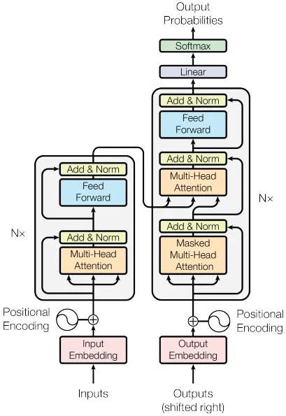
1. Inputs and Embeddings:

The bottom-most section of the diagram showcases how raw inputs are processed:

• Input Embedding: Textual data, in tokenized format, is transformed into dense vectors using embeddings. This acts as the initial representation of the data which the transformer will process.

• Positional Encoding: Since transformers don't inherently process data in sequence, positional encodings are added to ensure that the model retains information about the position of each token in a sequence.

2. Multi-Head Attention Mechanism:

A distinguishing feature of the transformer:

• Multi-Head Attention: Allows the model to focus on different parts of the input data simultaneously. It computes attention weights for different "heads", enabling the model to capture various aspects of the data.

• Masked Multi-Head Attention: Used primarily in the decoder section (as seen in the right-hand portion of the diagram). This ensures that while predicting a particular token, the model doesn't have access to future tokens.

3. Feed Forward Neural Networks:

Contained within each block of the architecture:

• Every layer in the transformer contains a feed-forward neural network, which operates independently on each position.

4. Add & Norm:

A crucial component for the model's stability and performance:

• After each main operation (attention or feed-forward), the output goes through an "Add & Norm" step which includes residual connections and layer normalization. This aids in preventing the vanishing gradient problem and ensures smoother training.

5. Linear Layers and Softmax:

The final steps before producing an output:

• Linear Layer: It transforms the output from the decoder's final layer.

• Softmax: Converts the raw output scores (logits) from the linear layer into probabilities. This is especially crucial when the model is used for tasks like classification.

6. Stacking:

As indicated by "N x" in the diagram, the transformer stacks these blocks multiple times, which allows it to learn more complex relationships and dependencies in the data.

Use case example

The Transformer architecture introduced in the paper revolutionized natural language processing tasks by utilizing self-attention mechanisms. The Language Model (LLM) based on this architecture can be thought of as a neural network model designed to understand and generate human language. It's particularly suited for tasks like machine translation, text summarization, and language generation.

1. Tokenization and Input Embeddings:

• The input sentence is first tokenized into subword or word-level tokens. Each token is represented as a vector using pre-trained embeddings (e.g., Word2Vec, GloVe).

• These embeddings are then transformed into input embeddings for the model. In the original Transformer, these embeddings have a fixed dimension.

2. Positional Encoding:

• Since the Transformer doesn't inherently understand the order of words in a sequence, positional encoding is added to the input embeddings.

• Positional encoding vectors are calculated based on the position of each token in the input sequence and added element-wise to the embeddings.

• This gives the model information about the relative positions of tokens in the sequence.

3. Encoder:

a. Self-Attention Mechanism: - The input embeddings with positional encodings are passed through multiple self-attention layers in parallel. - In each self-attention layer, queries, keys, and values are computed from the input embeddings. - Attention scores are calculated by taking the dot product of queries and keys, followed by scaling and applying a softmax function. - These attention scores determine how much each token should attend to other tokens in the same input sequence. - The weighted sum of values based on attention scores produces the attended representation for each token. - This mechanism allows the model to capture dependencies and relationships between words, emphasizing important connections.

b. Multi-Head Attention: - Multiple self-attention heads operate in parallel in each layer. - Each head has its own set of learned parameters, allowing it to focus on different aspects of the input. - The outputs of all heads are concatenated and linearly transformed to create the final attention output for that layer.

c. Residual Connection and Layer Normalization: - After each self-attention sub-layer, there is a residual connection that bypasses the sub-layer and a layer normalization step. - This helps in preventing the vanishing gradient problem during training and ensures smooth information flow through the network.

d. Feed-Forward Neural Network (FFN): - After self-attention, the output is passed through a feed-forward neural network. - The FFN consists of two linear transformations followed by an activation function (commonly ReLU) and another linear transformation. - This network captures complex, non-linear relationships between tokens.

e. Residual Connection and Layer Normalization (Again): - Similar to self-attention sub-layers, after the FFN, there is another residual connection and layer normalization.

4. Decoder:

• The decoder architecture closely resembles the encoder but with some differences. It also includes the following components:

a. Masked Self-Attention Mechanism: - In the decoder, self-attention is applied with a masking mechanism that prevents the model from attending to future positions in the output sequence.

b. Encoder-Decoder Attention: - In addition to the masked self-attention, the decoder also attends to the output of the encoder's final layer. - This allows the decoder to consider the entire input sequence while generating the output.

c. Residual Connections and Layer Normalization: - Similar to the encoder, residual connections and layer normalization are applied after each sub-layer in the decoder.

5. Output Generation:

• The final output from the decoder is passed through a linear layer followed by a softmax activation function.

• This produces a probability distribution over the vocabulary for each position in the output sequence.

• During training, the model is optimized to generate the correct target sequence by minimizing a suitable loss function like cross-entropy.

Information Flow:

• Information flows through the Transformer architecture in a hierarchical manner, with each layer capturing different levels of abstraction and dependencies between tokens.

• Self-attention mechanisms determine how much each token attends to other tokens in the input sequence, allowing the model to weigh their importance.

• The residual connections and layer normalization ensure that information can flow smoothly through the network without vanishing gradients.

• During decoding, the model attends to both the encoder's output and its own previously generated output to produce contextually relevant translations.

6. Conclusion

In the first post of "AI Odyssey" series, I went into the foundational aspects of Artificial Intelligence (AI) and Large Language Models (LLMs). I explored the basics of AI, the building blocks of neural networks, and took a look at the architecture that underpins modern LLMs, inspired by the groundbreaking paper "Attention Is All You Need."

As I go further into the world of AI, my next chapter will navigate the terrain of Deep Learning and Machine Learning Concepts. I’ll dissect various algorithms, dissect their strengths and weaknesses, and shed light on their practical applications.

It's important to note that this effort is a dynamic journey, fueled by my ongoing exploration and learning of AI. The purpose of this blog post series is twofold: to solidify my understanding of these complex subjects and, just as importantly, to share this knowledge with you.