E2: Journey into how Machines learn

Breaking Down ML

Introduction

As the digital landscape continuously change, introducing new paradigms, it’s a constant of a life for Software and Solution architect. The first chapter of my AI Odyssey went into Artificial Intelligence and Large Language Models, unravelling their foundational parts. My next stop is Machine Learning (ML). This realm is the fuel of the intelligence in AI.

Machine Learning, at its core, is about teaching machines to learn from data, to find patterns, and to make decisions (without awareness or consciousness). It's a foundational aspect in the broad field of AI, marking the initial steps towards equipping machines with a form of intelligence.

As an architect, exploring into ML means gaining a new perspective on the digital ecosystem. It's about understanding the mechanics that allow machines to exhibit human-like intelligence and using this knowledge to build strong, intelligent systems. Mastering ML concepts goes beyond theory, it's a practical journey to improve my architectural skills, to create systems that are not only efficient but also have the ability to learn, evolve, and adapt to the constantly changing digital environment.

This journey into ML and DL extends beyond just algorithms and models. It's about how I, as architect, can utilize learning machines to drive innovation, solve real-world issues, and develop systems that adapt to the dynamic digital age.

Unveiling Machine Learning (ML)

Machine Learning (ML) sits at the heart of modern computational innovation. It's not about programming explicit instructions, but rather feeding a system a large amount of data and allowing it to learn the patterns¹. This premise is simple yet powerful. As an architect, I find it amazing how a machine can be trained to discern patterns and make predictions or decisions based on data.

This is the crux of ML and where our exploration begins.

The realm of ML is broad, encapsulating various learning paradigms. It's essential from my reading to grasp these to comprehend how machines learn and adapt. The primary paradigms are:

Supervised Learning

Supervised learning is a type of Machine Learning paradigm where the model is trained on labelled data. The data is provided with the answer key, and the algorithm iteratively makes predictions on the training data and is corrected by the teacher (In this context, the term "teacher" metaphorically refers to the provided labels or the ground truth in the dataset), allowing the model to learn over time.

The Mathematics Behind it:

In Supervised Learning, we typically have a dataset of input-output pairs, denoted as

\((x 1 ​ ,y 1 ​ ),(x 2 ​ ,y 2 ​ ),...,(x n ​ ,y n ​ )\)

where x represents the input data and y represents the labels.

One common algorithm used in Supervised Learning is Linear Regression. The goal is to find the parameters that minimize the difference between the predicted outputs and the true outputs. Mathematically, it’s defined as “loss function”, usually the Mean Squared Error (MSE) loss.

Linear Regression is like finding the straight line that best fits or represents the relationship between house size and price. The closer this line is to the actual prices, the better, a fantastic explanation of the Linear Regression you can find it here

Understanding Linear Regression

The Mean Squared Error (MSE) is a way to measure how well the line fits the data by averaging the squares of the differences (errors) between the predicted prices and the actual prices. Our goal is to adjust the line to minimize these errors, resulting in the best possible predictions.

Real-World Use Case: Predicting House Prices

Let's consider a simplified scenario where I’m using a single feature (house size) to predict the house price. Our dataset consists of various house sizes and their corresponding price

Collecting and Preparing Data:

• Gather a dataset of house sizes and their prices.

• Split the data into a training set and a testing set.

Choosing a Model:

• Choose Linear Regression as our model since we're dealing with continuous data.

• n: The total number of data points (e.g., the number of houses you're considering).

• yi​: The actual value of the target variable for the i-th data point (e.g., the actual price of the i-th house).

• y^​i​: The predicted value of the target variable for the i-th data point (e.g., the price of the i-th house predicted by your model).

• ∑: This symbol represents summation, meaning you'll add up the squared differences for all n data points.

• (yi​−y^​i​)2: This part of the formula represents the squared difference between the actual value and the predicted value for each data point.

In simpler terms, we are finding the average of the squared differences between the actual values and the predicted values, which gives you a measure of the accuracy of your model.

1. Training the Model:

   • Use the training set to find the parameters that minimize the MSE loss.

2. Evaluating the Model:

   • Use the testing set to evaluate the model's performance.

   • Measure the accuracy using metrics like R-squared or Root Mean Squared Error (RMSE).

3. Making Predictions:

   • Now, given a new house size, use the learned parameters to predict its price.

4. Interpreting the Results:

   • Analyze how well the model generalizes to new, unseen data.

This process shows how Supervised Learning algorithms like Linear Regression can be used to make predictions on continuous data, thus aiding in better decision-making and system design from an architectural standpoint.

Unsupervised Learning

Unsupervised Learning (UL) is another realm of Machine Learning, where the algorithms are left on their own to discover and present the interesting structures in the data. Unlike Supervised Learning, there are no labels here, no teacher to correct the model. The model learns through observation and finds structures in the data on its own.

One classic example of Unsupervised Learning is clustering.

Clustering² is a technique used to group data points together based on certain similarities, without having prior knowledge of these groups. Imagine we have a dataset of different varieties of wines, each wine represents a data point with features like color, alcohol content, and sugar level.

data = {
    'Wine_Variety': ['Merlot', 'Chardonnay', 'Cabernet Sauvignon', 'Pinot Noir', 'Riesling', 'Sauvignon Blanc', 'Zinfandel'],
    'Color': ['Red', 'White', 'Red', 'Red', 'White', 'White', 'Red'],
    'Alcohol_Content': [13.5, 14.0, 13.8, 13.4, 11.5, 13.0, 14.5],  # in percentage
    'Sugar_Level': [1.5, 2.0, 1.2, 1.8, 2.5, 1.9, 2.2]  # scale from 1 to 3 (1-Dry, 2-Medium, 3-Sweet)
}

The essence of clustering lies in finding inherent groupings within the data. The algorithm explores the structure of the data to identify clusters of wines that share similar characteristics, essentially uncovering hidden patterns. This way, even without pre-defined labels, the wines are categorized into different groups, making the data more understandable and ready for further analysis.

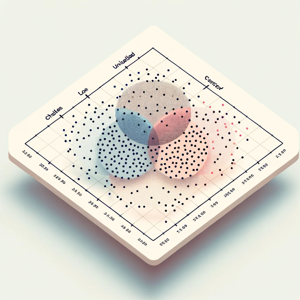
Probably the most popular clustering algorithm used in unsupervised machine learning and data analysis is K-means. The algorithm categorizes the data into K number of clusters. It works iteratively to assign each data point to one of K groups based on the features that are provided

Step 1: Initialization - Randomly initialize K centroids.

Step 2: Assignment - Assign each data point to the nearest centroid, and it becomes a member of that cluster.

Step 3: Update - Calculate the new centroid (mean) of each cluster.

Step 4: Repeat Steps 2 and 3 until there are no changes in the assignments or a maximum number of iterations is reached.

# File path: /your_directory/wine_clustering.py

# Importing necessary libraries
from sklearn.cluster import KMeans
from sklearn.preprocessing import LabelEncoder
import pandas as pd

# Wine dataset
data = {
    'Wine_Variety': ['Merlot', 'Chardonnay', 'Cabernet Sauvignon', 'Pinot Noir', 'Riesling', 'Sauvignon Blanc', 'Zinfandel'],
    'Color': ['Red', 'White', 'Red', 'Red', 'White', 'White', 'Red'],
    'Alcohol_Content': [13.5, 14.0, 13.8, 13.4, 11.5, 13.0, 14.5],
    'Sugar_Level': [1.5, 2.0, 1.2, 1.8, 2.5, 1.9, 2.2]
}
df_wine = pd.DataFrame(data)

# Converting the 'Color' column to numerical values
le = LabelEncoder()
df_wine['Color'] = le.fit_transform(df_wine['Color'])  # Red:1, White:0

# Defining the number of clusters
num_clusters = 3

# Creating the KMeans object and fitting it to the wine data
kmeans = KMeans(n_clusters=num_clusters, random_state=0).fit(df_wine[['Color', 'Alcohol_Content', 'Sugar_Level']])

# The labels of the clusters
labels = kmeans.labels_

# The centroids of the clusters
centroids = kmeans.cluster_centers_

# Adding the cluster labels to the original DataFrame
df_wine['Cluster'] = labels

# Now df_wine has an additional column 'Cluster' indicating the cluster each wine

In this code

1. The 'Color' column is converted to numerical values using the LabelEncoder from scikit-learn, where Red is encoded as 1 and White is encoded as 0.

2. The KMeans object is created and fitted to the wine data using the specified number of clusters (num_clusters = 3).

3. Cluster labels are generated and added to the original DataFrame in a new column called 'Cluster'.

Output Python One Compiler Code :

         Wine_Variety  Color  Alcohol_Content  Sugar_Level  Cluster
0              Merlot      0             13.5          1.5        1
1          Chardonnay      1             14.0          2.0        2
2  Cabernet Sauvignon      0             13.8          1.2        1
3          Pinot Noir      0             13.4          1.8        1
4            Riesling      1             11.5          2.5        0
5     Sauvignon Blanc      1             13.0          1.9        2
6           Zinfandel      0             14.5          2.2        1

The Mathematics Behind it:

The objective of K-means is to minimize the variance within each cluster and maximize the variance between different clusters. Mathematically, it’s defined as an objective function J that we aim to minimize

Algorithm

1. Clusters the data into k groups where k  is predefined.

2. Select k points at random as cluster centers.

3. Assign objects to their closest cluster center according to the Euclidean distance function.

4. Calculate the centroid or mean of all objects in each cluster.

5. Repeat steps 2, 3 and 4 until the same points are assigned to each cluster in consecutive rounds.

As an architect, the potential of uncovering hidden structures in data, which could be pivotal in designing intelligent systems that can discover and adapt to the underlying patterns in the ever-evolving digital landscape.

Reinforcement Learning

Reinforcement Learning (RL) is a type of learning where an agent learns how to behave in an environment by performing certain actions and observing the rewards of those actions. It's much like learning by trial and error. In RL, the agent receives feedback in the form of rewards or penalties, which it uses to adjust its behavior to achieve the maximum cumulative reward

Imagine I’m developing a wine recommendation system (our agent) to suggest wines to customers based on their past preferences. Each successful recommendation, where a customer buys or positively rates a wine, rewards our system, while unsuccessful recommendations penalize it. Over time, our system learns to make better recommendations, maximizing customer satisfaction and, by extension, sales.

import numpy as np

# Define the states, actions, rewards, and other parameters
states = [...]  # e.g., different customer profiles
actions = [...]  # e.g., different wine recommendations
rewards = np.zeros((len(states), len(actions)))  # initialize rewards matrix
q_values = np.zeros((len(states), len(actions)))  # initialize Q-values matrix
alpha = 0.1  # learning rate
gamma = 0.9  # discount factor

# Simulate the Q-learning process
for episode in range(1000):  # assume 1000 episodes
    state = np.random.choice(states)  # start with a random state
    while True:
        action = np.argmax(q_values[state, :] + np.random.randn(1, len(actions)) * (1./(episode+1)))  # choose an action
        reward = rewards[state, action]  # get the reward
        next_state = ...  # determine the next state
        # Update the Q-value
        q_values[state, action] = q_values[state, action] + alpha * (reward + gamma * np.max(q_values[next_state, :]) - q_values[state, action])
        state = next_state  # move to the next state
        if ...:  # check if the episode ends
            break

In this code snippet, I initialize our Q-values and simulate the Q-learning process over 1000 episodes to improve the wine recommendation system. With each episode, the Q-values are updated, and the recommendation policy improves, leading to better wine recommendations over time.

The Mathematics Behind it:

In RL, the agent uses a strategy known as a policy to decide its actions. One common approach is using a Q-Learning algorithm, which estimates the total expected rewards for each action in each state. The Q-value for a particular state-action pair is updated using the formula:³

• s and s′ are the current and next states,

• a and a′ are the current and potential future actions,

• r is the immediate reward,

• α is the learning rate (how much we update our Q-value),

• γ is the discount factor (how much we value future rewards).

Architectural Insights

In my journey, especially in commerce projects, platforms like Salesforce Commerce Cloud and SAP Commerce have been my playgrounds. These platforms leverage machine learning extensively to power their recommendation and promotion engines, providing a more tailored shopping experience. For instance, on Salesforce Commerce Cloud, the Einstein AI provides personalized recommendations by analyzing shopper data and behaviors using

• Linear Regression: For predicting numerical values like sales forecasts.

• Classification Algorithms: For categorizing data into various classes. Algorithms like Random Forest, SVM, and Decision Trees might be employed.

Designing systems around Machine Learning (ML) like this one calls for a understanding of scalability, efficiency, and deployment strategies.

Scalability isn’t just about handling increased load; it's about ensuring the ML models can be re-trained with larger datasets to improve accuracy over time. Efficiency touches on optimizing computational resources, minimizing latency, and ensuring the ML algorithms are fine-tuned for performance. Deployment strategies should be crafted to allow for smooth transitions, version control of models, and robust monitoring to catch anomalies early.

Training Scalability

Distributed Training⁴

This is a technique that partitions the data and model across multiple nodes to parallelize the computational workload. From an architectural standpoint, it leverages horizontal scaling, capitalizing on data parallelism and model parallelism techniques. By distributing the model's parameters and layers across various GPUs or even across multiple servers, we can achieve a significant reduction in training time. This enables organizations to expedite their time-to-market and handle large-scale, high-dimensional data efficiently. It's critical to integrate Distributed Training into the architecture from the get-go, ensuring seamless scalability while keeping an eye on network latency and data synchronization overhead.

Data Parallelism

Data Parallelism involves distributing the dataset across multiple nodes (usually GPUs) and training a replica of the model on each node. Each node computes the gradients based on its subset of the data, which are then aggregated to update the model.

How It Works:

1. Partition the dataset into smaller batches.

2. Distribute the batches across multiple GPUs.

3. Each GPU computes the forward and backward pass using its subset of data.

4. Aggregate the gradients from all GPUs.

5. Update the model parameters.

Pros:

• Simplicity: Easier to implement and manage.

• Batch Size: Allows for larger effective batch sizes, which can lead to a more stable and improved convergence.

• Scalability: Highly scalable as you can add more GPUs to handle larger datasets.

Cons:

• Communication Overhead: Requires synchronization to aggregate gradients, which can be bandwidth-intensive.

• Limited by Dataset: If the dataset is too small, it may not benefit much from data parallelism.

Model Parallelism

Definition:
Model Parallelism involves splitting the model itself across multiple nodes. Each node is responsible for computing the forward and backward passes for its part of the model.

How It Works:

1. Divide the model layers or parameters across multiple GPUs.

2. Each GPU computes the forward and backward pass for its part of the model.

3. Communicate the intermediate outputs between GPUs as needed.

Pros:

• Memory Efficiency: Allows for training of models that would not fit into the memory of a single GPU.

• Complex Models: Enables training of more complex models.

Cons:

• Communication Overhead: Requires frequent communication between GPUs to share intermediate outputs.

• Implementation Complexity: More challenging to implement and manage compared to data parallelism.

Data Parallelism vs Model Parallelism

1. Ease of Implementation:

   • Data Parallelism: Generally easier to implement.

   • Model Parallelism: Requires more intricate handling of model layers and states.

2. Memory Utilization:

   • Data Parallelism: Can be limited by the memory of a single GPU for storing the model.

   • Model Parallelism: More efficient in using memory for very large models.

3. Communication Overhead:

   • Data Parallelism: Involves less frequent but larger data transfers (aggregating gradients).

   • Model Parallelism: Requires more frequent but smaller data transfers (intermediate layer outputs).

4. Scalability:

   • Data Parallelism: Scales well with larger datasets.

   • Model Parallelism: Scales well with model complexity.

5. Use-Cases:

   • Data Parallelism: Effective for large-scale but simpler models.

   • Model Parallelism: Necessary for complex models with many parameters that won't fit into a single GPU's memory.

1. Strategy: Data Sharding

   • Pros: Efficient handling of large datasets, reduces memory load.

   • Cons: Requires consistent data distribution, potential loss of inter-shard information.

Conclusion

In this episode, I've broken down the core concepts of Machine Learning, crucial for any architect aiming to leverage AI within system designs. The discussion around design considerations for ML systems, focusing on scalability, is fundamental for the architectural planning of robust, intelligent systems. The next episode will further this exploration into Deep Learning, extending our toolkit and understanding for designing AI-driven architectures.

Engage and with this learning journey; share your insights or ask questions in the comments below. If you found value in this exploration, share it within your network. Stay tuned for the next episode where we'll delve deeper into Deep Learning, further broadening our architectural horizon in the AI realm. Subscribe now to stay updated!

1. https://www.microsoft.com/en-us/research/uploads/prod/2006/01/Bishop-Pattern-Recognition-and-Machine-Learning-2006.pdf

2. https://developers.google.com/machine-learning/clustering/clustering-algorithms

3. https://static1.squarespace.com/static/5ff2adbe3fe4fe33db902812/t/6009dd9fa7bc363aa822d2c7/1611259312432/ISLR+Seventh+Printing.pdf

4. https://storage.googleapis.com/pub-tools-public-publication-data/pdf/40565.pdf